Ordinal Regression Models in Psychology: A Tutorial をRでやってみる。データは https://osf.io/cu8jv/ にある stemcell.csv を使う。
まずデータを読んでみる。
> stemcell = read.csv("stemcell.csv", stringsAsFactors=TRUE)
> str(stemcell)
'data.frame':	829 obs. of  3 variables:
 $ belief: Factor w/ 3 levels "fundamentalist",..: 1 1 1 1 1 1 1 1 1 1 ...
 $ rating: int  1 1 1 1 1 1 1 1 1 1 ...
 $ gender: Factor w/ 2 levels "female","male": 1 1 1 1 1 1 1 1 1 1 ...
> levels(stemcell$belief)
[1] "fundamentalist" "liberal"        "moderate"
table(stemcell$belief, stemcell$rating)

                   1   2   3   4
  fundamentalist  55 119  54  40
  liberal        122 113  31  23
  moderate        71 135  41  25
いくつか論文と比べて違うところがある。まず、stemcell$belief のレベルは基準となる "moderate" が一番左に来なければいけないのにそうなっていない。あと、テーブルをみると1、2、3、4がまったく逆に並んでいる。次のようにすれば直る。
> stemcell$belief = relevel(stemcell$belief, ref="moderate")
> stemcell$rating = 5 - stemcell$rating
> levels(stemcell$belief)
[1] "moderate"       "fundamentalist" "liberal"
> table(stemcell$belief, stemcell$rating)

                   1   2   3   4
  moderate        25  41 135  71
  fundamentalist  40  54 119  55
  liberal         23  31 113 122
さて、いよいよ brms パッケージを使う。論文通りにやればいいが、marginal_effects() は conditional_effects() が新しい名前のようだ。
> install.packages("brms")
> library(brms)
> fit_sc1 = brm(formula=rating ~ 1 + belief, data=stemcell, family=cumulative("probit"))
...(中略)...
> summary(fit_sc1)
 Family: cumulative
  Links: mu = probit
Formula: rating ~ 1 + belief
   Data: stemcell (Number of observations: 829)
  Draws: 4 chains, each with iter = 2000; warmup = 1000; thin = 1;
         total post-warmup draws = 4000

Regression Coefficients:
                     Estimate Est.Error l-95% CI u-95% CI Rhat Bulk_ESS Tail_ESS
Intercept[1]            -1.25      0.08    -1.41    -1.09 1.00     2914     3078
Intercept[2]            -0.64      0.07    -0.78    -0.50 1.00     3484     3401
Intercept[3]             0.57      0.07     0.43     0.71 1.00     3763     3452
belieffundamentalist    -0.24      0.09    -0.43    -0.06 1.00     3393     2590
beliefliberal            0.31      0.09     0.13     0.49 1.00     3426     3165

Further Distributional Parameters:
     Estimate Est.Error l-95% CI u-95% CI Rhat Bulk_ESS Tail_ESS
disc     1.00      0.00     1.00     1.00   NA       NA       NA

Draws were sampled using sampling(NUTS). For each parameter, Bulk_ESS
and Tail_ESS are effective sample size measures, and Rhat is the potential
scale reduction factor on split chains (at convergence, Rhat = 1).
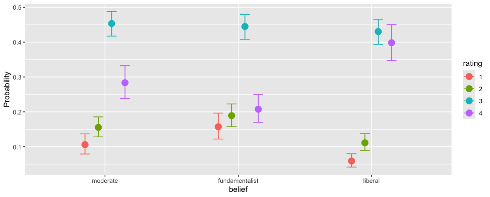
> conditional_effects(fit_sc1, 'belief', categorical=TRUE)
比較として、単に1〜4それぞれの割合とその95%信頼区間(binom.test()$conf.int)を描いてみる:
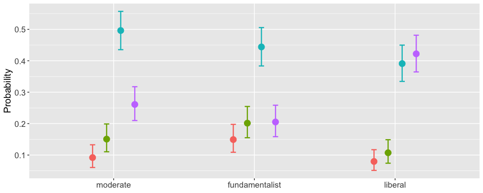
これらがわかりやすいかどうかは微妙だ。単に HH パッケージで帯グラフにしてみよう。
library("HH")
plot.likert(table(stemcell$belief, stemcell$rating),
            main="Opinions about funding stem-cell research")
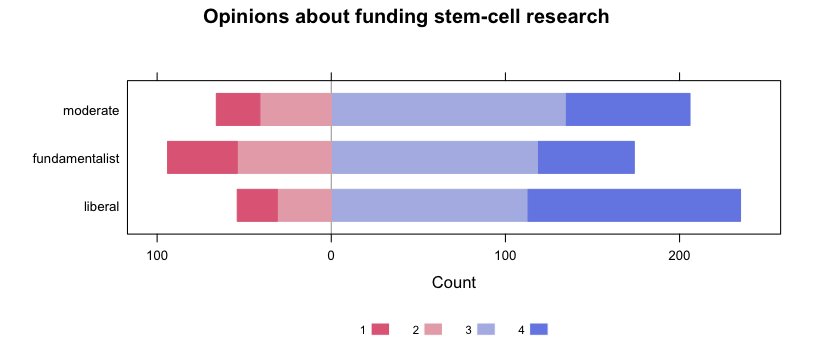
リベラル派の方が幹細胞研究に資金を出すべきだという人が多いことがわかる。